SCIMES tutorial
In this tutorial we will show the steps necessary to obtain the segmentation of
the Orion-Monoceros dataset (orion_12CO.fits)
presented in the SCIMES paper. Most of this tutorial is collected in the
script orion2scimes.py.
Building the dendrogram and the structure catalog
First, we need to compute the dendrogram and its related catalog,
i.e. the inputs of SCIMES. In this example we are dealing with
real observations. Therefore, we have to open a FITS file by using,
for example, astropy :
>>> from astropy.io import fits
>>> hdu = fits.open('orion_12CO.fits')[0]
>>> data = hdu.data
>>> hd = hdu.header
Afterward the dendrogram can be computed:
>>> from astrodendro import Dendrogram
>>> d = Dendrogram.compute(data)
the astrodendro.dendrogram.Dendrogram class has various tuning parameters. To explore them and their meaning, please refer to: Computing and exploring dendrograms.
The dendrogram of Orion-Monoceros can be simply obtained using the following parameters:
>>> sigma = 0.3 #K, noise level
>>> ppb = 1.3 #pixels/beam
>>> from astrodendro import Dendrogram
>>> d = Dendrogram.compute(data, min_value=sigma, min_delta=2*sigma, min_npix=3*ppb)
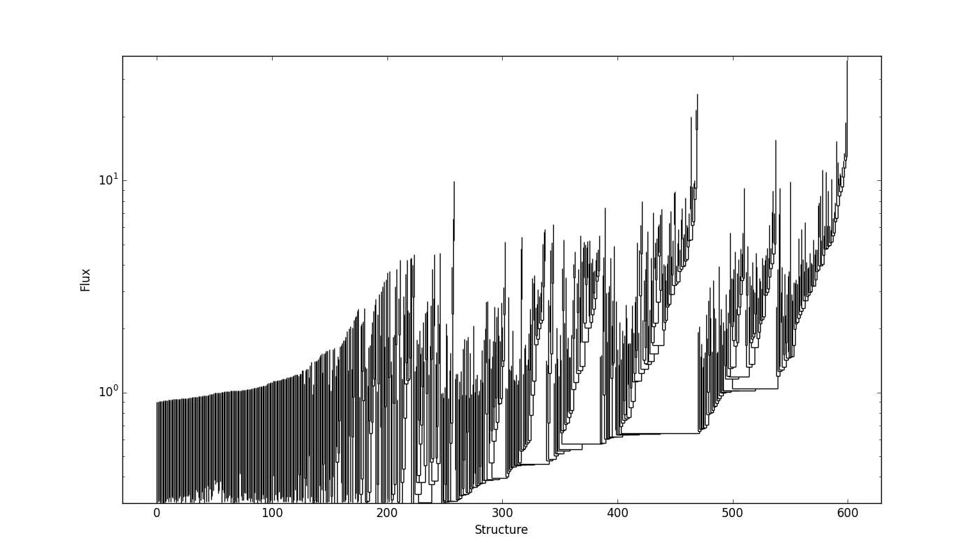
and it looks like:
SCIMES applies the spectral clustering based on the properties of
all structures within the dendrogram. The dendrogram catalog
can be obtained by the ppv_catalog() or pp_catalog() functions, for example:
>>> from astrodendro import ppv_catalog
>>> from astropy import units as u
>>> metadata = {}
>>> metadata['data_unit'] = u.Jy
>>> cat = ppv_catalog(d, metadata)
Further information about the dendrogram catalog functions can be found here: Making a catalog.
Clustering the dendrogram
The clustering of the dendrogram is obtained through the
SpectralCloudstering class which requires as inputs
the dendrogram and its related catalog:
>>> from scimes import SpectralCloudstering
>>> dclust = SpectralCloudstering(d, cat)
By default, the clustering is performed on the aggregate affinity matrix given by the element-wise multiplication of the luminosity and the volume matrix. If instead you want to perform the clustering based on volume only, ignoring luminosity, this can be achieved by setting:
>>> dclust = SpectralCloudstering(d, cat, criteria = ['volume'])
or if only the luminosity matrix is needed:
>>> dclust = SpectralCloudstering(d, cat, criteria = ['luminosity'])
The SpectralCloudstering class provides several
optional inputs:
criteria: the criteria used to cluster the dendrogram. The names listed must correspond to structure properties present in the catalog. In principle, any (meaningful) catalog property can work as clustering criterion. The user can provide as many criteria as needed,SCIMESwill generate affinity matrices for each of them and the aggregate matrix for the final clustering.user_k: the number of clusters expected can be provided as an input. In this case,SCIMESwill not make any attempt to guess it from the affinity matrix.user_ams: if clustering based on a different property than volume and luminosity is wanted, this can be obtained by providing a user defined affinity matrix. This matrix needs to be ordered according to the dendrogram leaves indexing. Several matrices based on various properties can be provided all together;SCIMESaggregates them and generates the clustering based on all these properties.user_scalpars: the scaling parameters of the affinity matrices can be provided as input. The scaling parameters are used to suppress some affinity values of the matrix and enhance others by rescaling the matrices with a Gaussian kernel. Also, this operation normalizes the matrices and prompts the user whether the matrices should be aggregated or this step should be skipped, proceeding directly to the clustering. The choice of the scaling parameters might influence the final result. If not provided,SCIMESestimates them directly from the affinity matrices.user_iter: number of k-means iterations to be performed. By default,user_iter = 100. This value can be increased, increasing the k-means stability and the computation time.rms: the noise level of the observation. If provided,SCIMEScalculates the scaling parameter above a certain signal-to-noise ratio threshold within the dendrogram. The threshold expressed is expressed ass2nlim*rms.s2nlimis set by default to 3, but it can also by provided as input. THIS IS A STRONGLY RECOMMENED INPUT SINCE IT INCREASES THE STABILITY OF THE CODE.save_isol_leaves: by definition single leaves do not form clusters, since clusters are constituted by at least two objects. Therefore, they are eliminated by default from the final cluster counts. For some applications, as in case of low resolution observations, single leaves might represent relevant entities that need to be retained. This keyword forcesSCIMESto consider unclustered and isolated leaves (e.g. without parent, trunks) as independent clusters that will appear in the final cluster index catalog.save_clust_leaves: when triggered it forcesSCIMESto retain asclustersthe intra-clustered leaves usually discarded as noise. This keyword will not include the isolated leaves without parents, assave_isol_leavesoption.save_all_leaves: it triggers bothsave_isol_leavesandsave_clust_leavesoptions.save_branches: when a cluster of leaves cannot be attributed to a single isolated branch containing only the leaves of the cluster, the cluster leaves are pruned until this condition is satisfied. The final branch representing the cluster will have the larger amout of leaves of the selected cluster. During this operation several isolated branches within the same cluster might result unassignible. By triggeringsave_branches, those branches are retained and assigned to separed objects.save_all_leaves: it triggers bothsave_all_leavesandsave_branchesoptions.
As an example, we run SpectralCloudstering on the Orion-Monoceros
dataset, using the “volume” matrix only without including distance
information. In this case SCIMES prints:
>>> Running SCIMES
>>> WARNING: adding luminosity = flux to the catalog.
>>> WARNING: adding volume = pi * radius^2 * v_rms to the catalog.
>>> WARNING: clustering will be performed on the Volume matrix only
The first two WARNINGs are related to the fact that in the original
implementation of the ppv_catalog(), “volume” and “luminosity” are not
present. SCIMES calculates them using the properties within the
catalog and adds them to the catalog. The third WARNING relates to the
fact that the clustering will be performed only on the “volume” matrix.
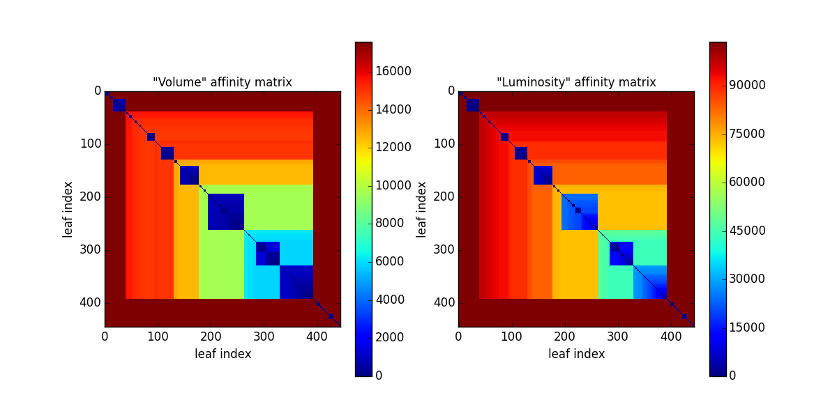
Firstly, SCIMES proceeds to calculate the affinity matrices:
>>> - Creating affinity matrices
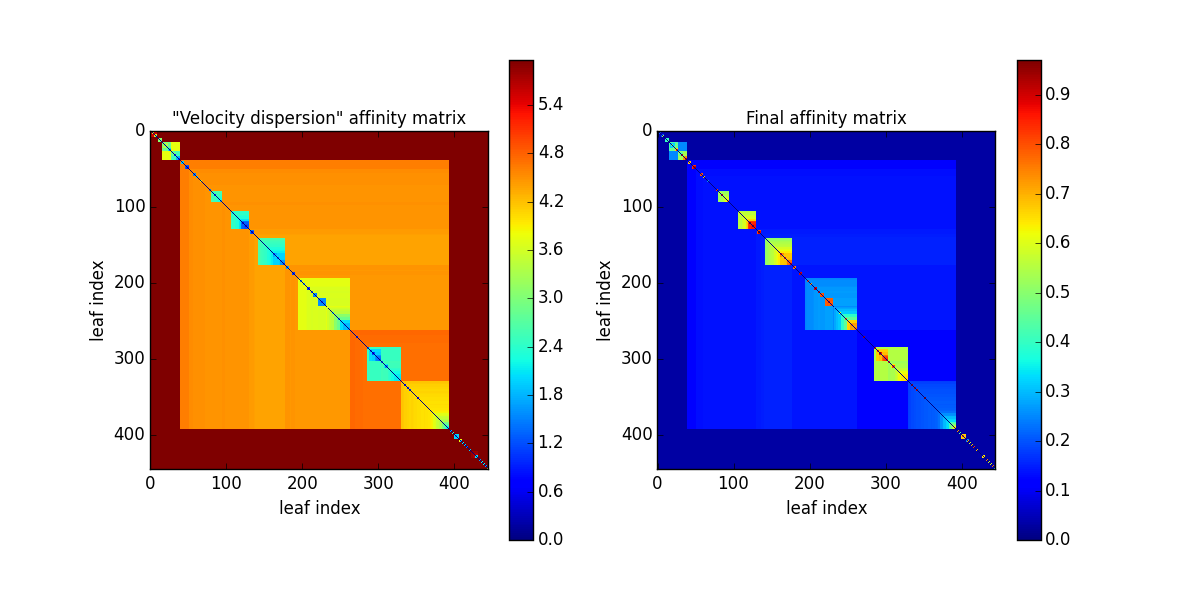
If the keyword blind == False the affinity matrices are visualized:
Then the spectral clustering starts. Only the “volume” matrix (matrix 0) is rescaled. The estimated scaling parameter is shown.
>>> - Start spectral clustering
>>> -- Smoothing  0  matrix
>>> -- Estimated scaling parameter: 3643.23718741
Afterwards, if blind == False, the rescaled matrix is also
visualized:
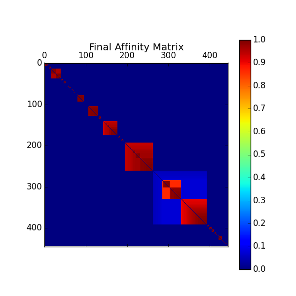
In the case whose the “luminosity” clustering criterion is also selected, the final matrix is the product of the rescaled “volume” and “luminosity” matrices.
The number of cluster to find is first guessed from the number of blocks present along the main diagonal of the final affinity matrix. This number is further optimazed by calculating the value of the “silhouette” (see next Section) for 30 clustering configurations around the guessed value. The “silhouette” value of the best configuration is also printed.
>>> -- Guessed number of clusters = 42
>>> -- Best cluster number found through SILHOUETTE ( 0.985594230523 )=  43
At this point the spectral clustering finds the best assessment of dendrogram leaves within 43 clusters. However, some clusters cannot be assigned to specific branches within the dendrogram and they are eliminated from the final cluster counts; the cluster number 2 and 13 are considered “unassignable”. This operation is called “cluster cleaning”.
>>> -- Unassignable cluster  2
>>> -- Unassignable cluster  13
The final number of clusters for the Orion-Monoceros dendrogram using the “volume” criterion is 41:
>>> -- Final cluster number (after cleaning) 41
If, for example, the save_all option is selected, the following messages
will appear:
>>> SAVE_BRANCHES triggered, all isolated branches will be retained
>>> -- Final cluster number (after cleaning) 41
>>> -- Final clustering configuration silhoutte 0.541521
>>> SAVE_ISOL_LEAVES triggered. Isolated leaves added.
>>> -- Total cluster number 196
>>> SAVE_CLUST_LEAVES triggered. Unclustered leaves added.
>>> -- Total cluster number 257
Once the unclustered branches are added, the silhoutte is recalculated for the new clustering configuration. Since the configuration obtained with the added clusters is not ideal, the silhouette value can be largely reduced.
Clustering results
The main output of the algorithm, clusters, is a list of dendrogram
indices representing the relevant structures within the dendrogram according
to the scale of the observation and the affinity criteria used. In the
case of Orion-Monoceros, the properties of the structures are the
equivalent to “Giant Molecular Clouds”. Those structures are already
present in the dendrogram. The hierarchy can be accessed
following the instructions on the astrodendro documentation page,
while their properties and statistics are collected in the dendrogram pp or ppv catalog.
SCIMES provides other outputs that result from the
clustering analysis:
affmats: numpy arrays containing the affinity matrices produced by the algorithm or provided as inputs by the user. The indices of those matrices represent theleavesof the dendrogram permuted in order to make the possible matrix block structure emerge. The permutation, however, does not influence the following spectral embedding.escalpars: list containing the estimated scale parameters from the clustering analysis associated with the different input affinity matrices. Scaling parameters represent maximal properties (by defaultvolumeandluminosity, orflux) that the final structures tend to have.silhouette: float showing the silhouette of the selected clustering configuration. This value ranges between 0 and 1 and represents the goodness of the clustering, where values close to 0 indicate poor clustering, while values close to 1 indicate well separated clusters (i.e. good clustering)
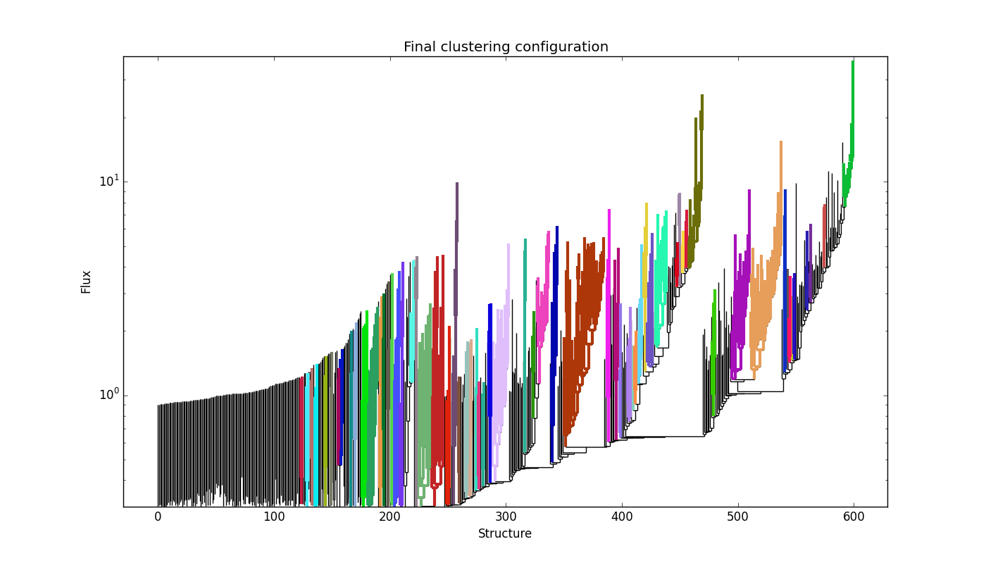
SCIMES visualizes the clusters within the dendrogram throught the
plot_tree method of astrodendro. Each cluster is indicated
with a different random color. Following the example in the previous
Section, this can be done through:
>>> dclust.showdendro()
The result for the Orion-Monoceros dendrogram is:
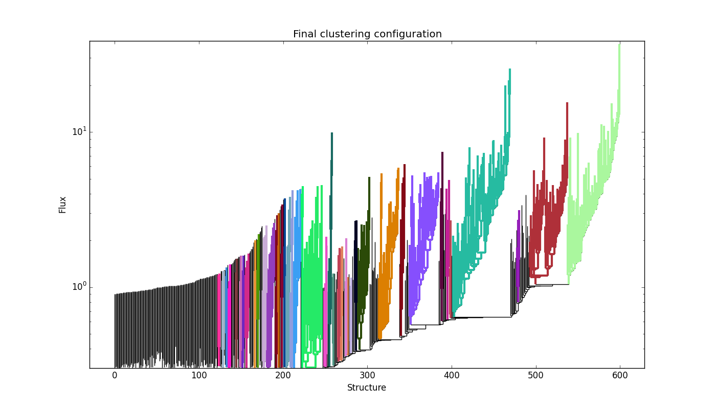
where each color indicates a single cluster/relevant object within the dendrogram.
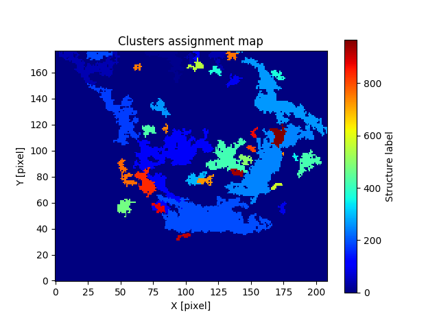
Together, SCIMES generates the assignment cube of the clouds
through the get_mask
method of astrodendro. Pixels within a given cloud are labeled
with a number related to the index of the dendrogram. This is automatically generated by the algorithm which produced the cubes for
identified clusters (dclust.clusters_asgn), leaves (dclust.leaves_asgn), and trunks (dclust.trunks_asgn) structures as astropy.io.fits.hdu.image.PrimaryHDU type. The collapsed version of the cluster assignment cube looks like:
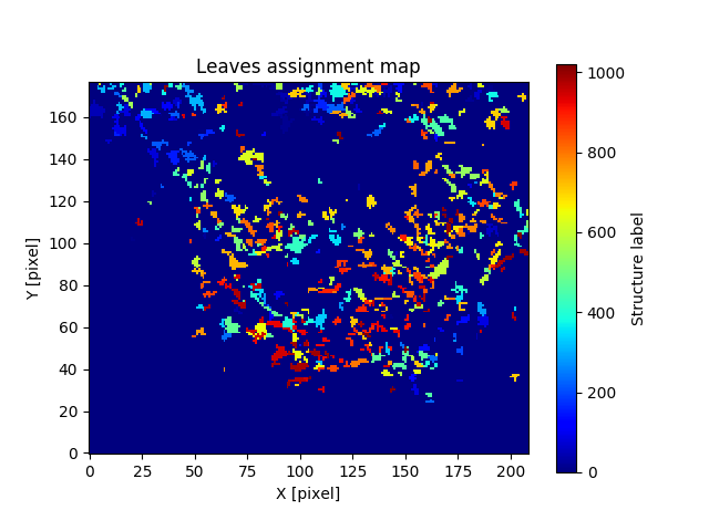
For the leaves assignment cube:
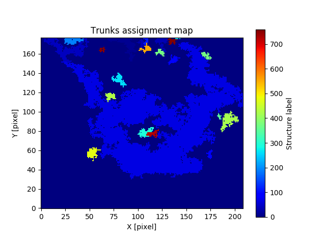
And for the trunks assignment cube:
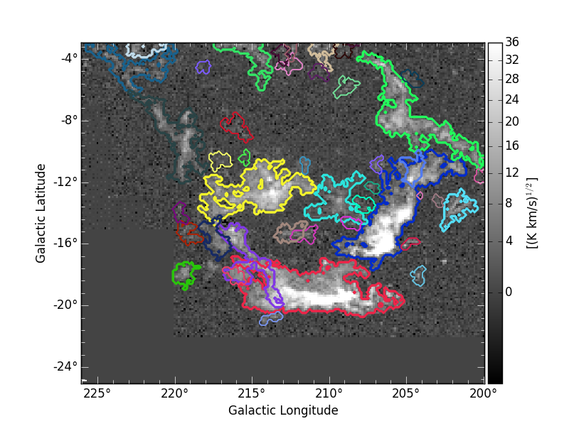
A nice representation of the decomposed objects might be obtained by using APLpy. Here the contours represent the identitied clusters:
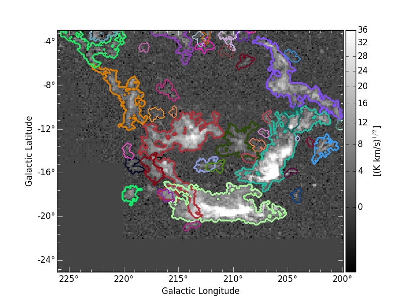
where the integrated intensity map can be downloaded from orion_12CO_mom0.fits.
At the same time the catalog is updated with some useful information regarding the structure type and its place within the dendrogram hierarchy. The added information for a given structure are the following:
parent: integer indicating the number of the parental structure. -1 is set for a structure without parent (trunk).ancestor: integer indicating the number of the structure at the bottom of the hierarchy of the given structure. The ancestor for a structure at the bottom of the hierarchy is itself.n_leaves: integer indicating the number of descendant of the given structure.type: string, ‘T’ indicates that the structure is a trunk or a branch without parent; ‘B’ indicates that the structure is branch with parent; ‘L’ indicates that the structure is a leaf.
Difference between pixel and physical property-based segmentation
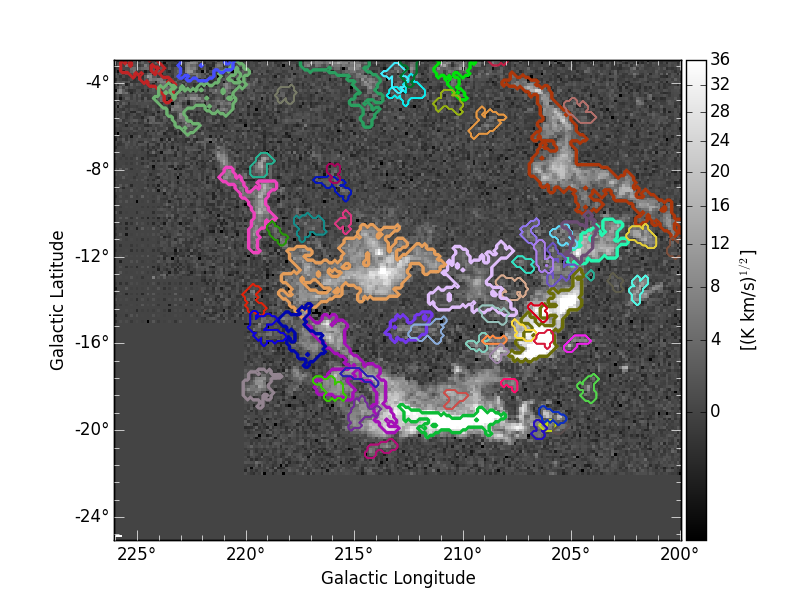
The above segmentation of the Orion-Monoceros dataset has been obtain using pixel-based properties. Nevertheless, if distances are know those can be attributed to every structrure within the dendrogram in order to provide segmentations based on the physical properties of the structures. By doing that, the “volume” criterion assume the units pc2 km/s. The objects obtained in this way are very similar to the ones decomposed using the pixel-based “volume”. Nevertheless, NGC2149 and Monoceros are separated:
Affinity matrix choice
By default SCIMES deals with the “volume” and “luminosity”
matrices. Nevertheless, every affinity matrix can be provided by the
user in order to obtain segmentation based on the desired property of
the ISM. This operation is generally made through the user_ams keyword.
However, SCIMES works well with monotonic and block
diagonal matrices, and might misbehave when non-monotonic and strictly
continous criteria are provided. In this example we show the
segmentation of the Orion-Monoceros dataset using the “velocity
dispersion” of the structures. The full run of SCIMES provides:
>>> - Creating affinity matrices
>>> - Start spectral clustering
>>> -- Rescaling  0  matrix
>>> -- Estimated scaling parameter: 2.0795701609
>>> -- Guessed number of clusters = 49
>>> -- Best cluster number found through SILHOUETTE ( 0.783614320248 )=  59
>>> -- Final cluster number (after cleaning) 66
In particular, the decomposed structures of the Orion-Monoceros dataset have a characteristic “velocity dispersion” of 2 km/s. However, the silhouette (~0.78) is not very high indicating a not optical clustering for this criteria. Moreover, the block in the affinity matrix are not well defined:
and the dendrogram branches appear overdivided:
providing:
This indicates that the structures in Orion-Monoceros are not highly separated along the line of sight and that, in general, the velocity dispersion is not a good criterion for this dataset.
SCIMES behaviour at low resolution
SCIMES is designed to find well resolved objects, constituted by
several resolution elements. Nevertheless, it might be applied also to low
resolution observations. In this case the code essentially behaves as
a “clump-finder”. When working at low resolution, the savesingles
keyword might be necessary, though (see above). In this example, the
Orion-Monoceros dataset has been smoothed to a resolution of 10 pc
(i.e. approximately a factor 10 lower than the original
resolution). The following image show the result of SCIMES run.
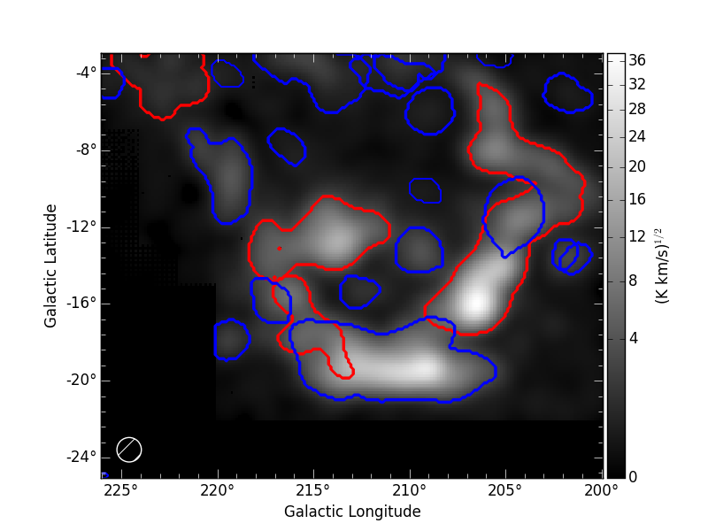
Red contours indicate objects that have been decomposed by SCIMES
using the default settings. Blue contours indicates, instead, the
additional objects retained by enabling the savesingles
keyword. This keyword forced SCIMES to keep single leaves in the
final cluster catalog, and allow to decomposed some notable clouds (as
Monoceros, the Crossbones, and the Scissor) that at this resolution
are constituted by a single leaf, therefore erased by default.